
Gaussian Process, not quite for dummies
Published:
Before diving in
For a long time, I recall having this vague impression about Gaussian Processes (GPs) being able to magically define probability distributions over sets of functions, yet I procrastinated reading up about them for many many moons. However, as always, I’d like to think that this is not just due to my procrastination superpowers. Whenever I look up “Gaussian Process” on Google, I find these well-written tutorials with vivid plots that explain everything up until non-linear regression in detail, but shy away at the very first glimpse of any sort of information theory. The key takeaway is always,
A Gaussian process is a probability distribution over possible functions that fit a set of points.
While memorising this sentence does help if some random stranger comes up to you on the street and ask for a definition of Gaussian Process – which I’m sure happens all the time – it doesn’t get you much further beyond that. In what range does the algorithm search for “possible functions”? What gives it the capacity to model things on a continuous, infinite space?
Confused, I turned to the “the Book” in this area, Gaussian Processes for Machine Learning by Carl Edward Rasmussen and Christopher K. I. Williams. I have friends working in more statistical areas who swear by this book, but after spending half an hour just to read 2 pages about linear regression I went straight into an existential crisis. I’m sure it’s a great book, but the math is quite out of my league.
So what more is there? Thankfully I found the above lecture by Dr. Richard Turner on YouTube, which was a great introduction to GPs, and some of its state-of-the-art approaches. After watching this video, reading the Gaussian Processes for Machine Learning book became a lot easier. So I decided to compile some notes for the lecture, which can now hopefully help other people who are eager to more than just scratch the surface of GPs by reading some “machine learning for dummies” tutorial, but don’t quite have the claws to take on a textbook.
Acknowledgement: the figures in this blog are from Dr. Richard Turner’s talk “Gaussian Processes: From the Basic to the State-of-the-Art”, which I highly recommend! Have a lookie here: Portal to slides.
Motivation: non-linear regression
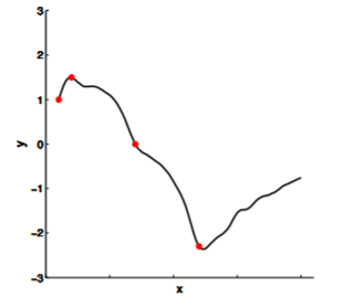
Of course, like almost everything in machine learning, we have to start from regression. Let’s revisit the problem: somebody comes to you with some data points (red points in image below), and we would like to make some prediction of the value of $y$ with a specific $x$.
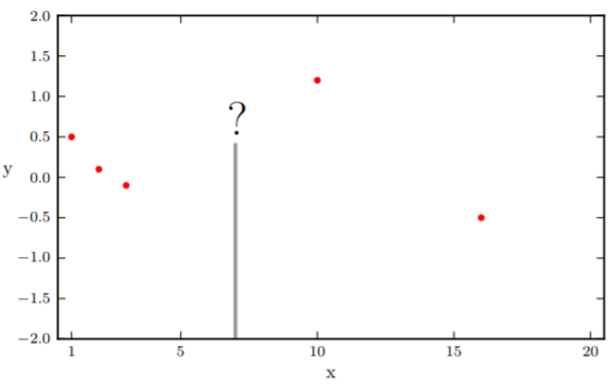
In non-linear regression, we fit some nonlinear curves to observations. The higher degrees of polynomials you choose, the better it will fit the observations.
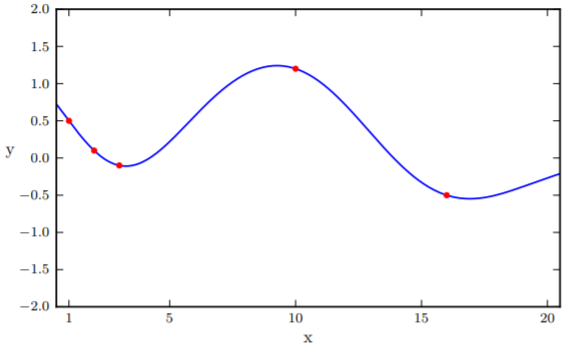
This sort of traditional non-linear regression, however, typically gives you one function that it considers to fit these observations the best. But what about the other ones that are also pretty good? What if we observed one more points, and one of those ones end up being a much better fit than the “best” solution?
To solve this problem, we turn to the good Ol’ Gaussians.
The world of Gaussians
Recap
Here we cover the basics of multivariate Gaussian distribution. If you’re already familiar with this, skip to the next section 2D Gaussian Examples.
The Multivariate Gaussian distribution is also known as the joint normal distribution, and is the generalisation of the univariate Gaussian distribution to high dimensional spaces. Formally, the definition is:
A random variable is said to be k-variate normally distributed if every linear combination of its k components have a univariate normal distribution.
Mathematically, $X = (X_1, …X_k)^T$ has a multivariate Gaussian distribution if $Y=a_1X_1 + a_2X_2 … + a_kX_k$ is normally distributed for any constant vector ${a} \in \mathcal{R}^k$.
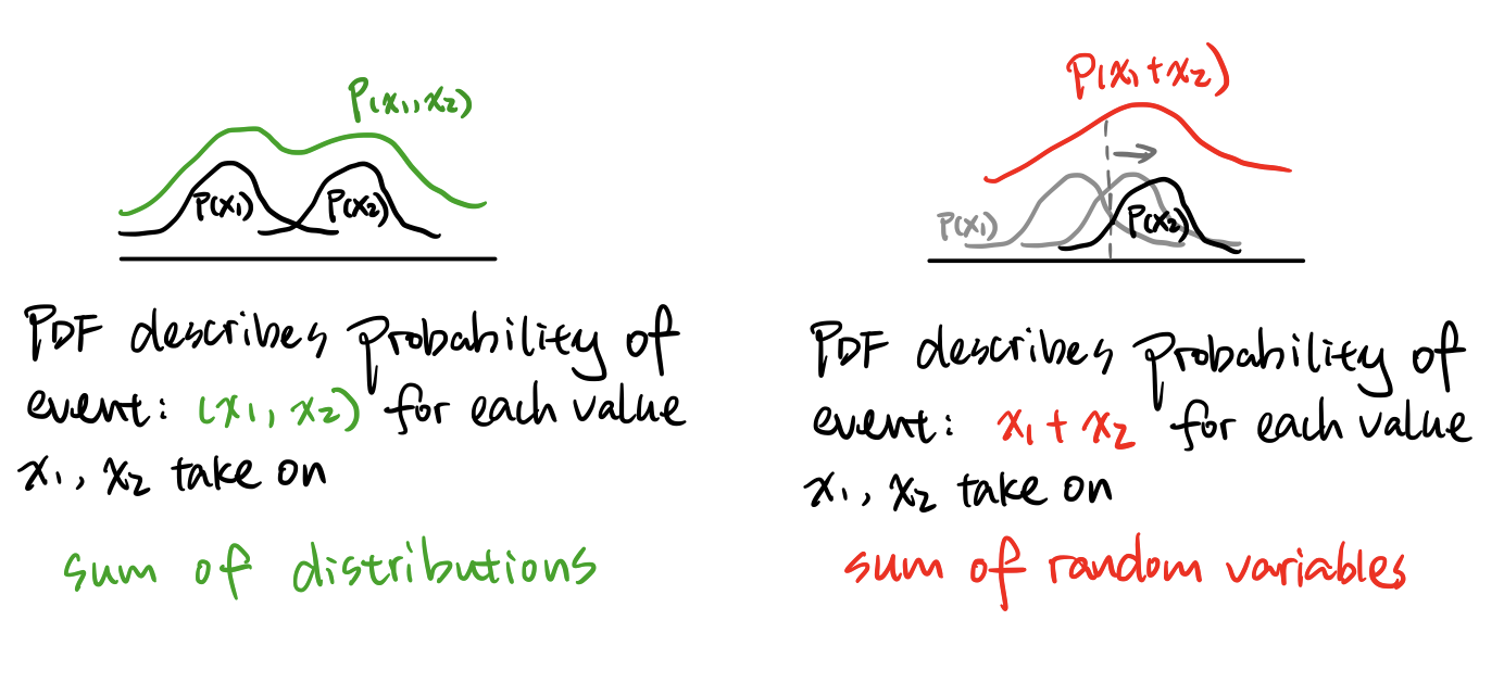
Note: if all k components are independent Gaussian random variables, then $X$ must be multivariate Gaussian (because the sum of independent Gaussian random variables is always Gaussian).
_Another note: sum of random variables is different from sum of distribution – the sum of two Gaussian distributions gives you a Gaussian mixture, which is not Gaussian except in special cases. _
2D Gaussian Examples
Covariance matrix
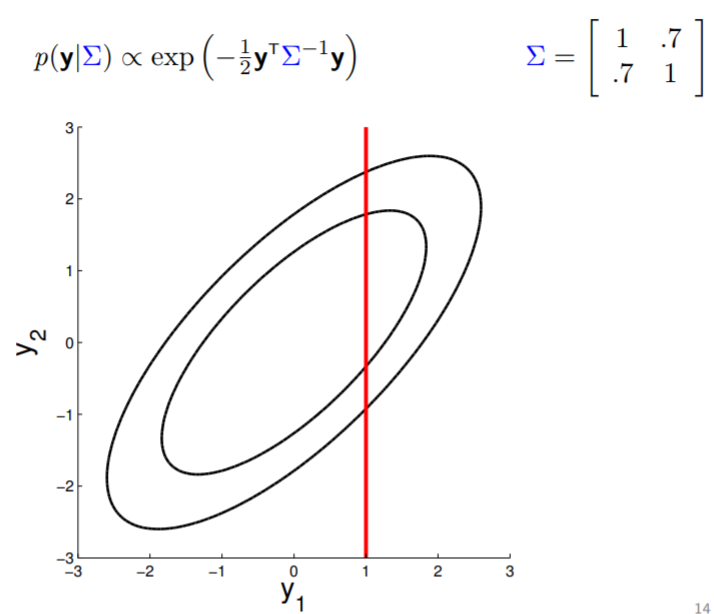
Here is an example of a 2D Gaussian distribution with mean 0, with the oval contours denoting points of constant probability.
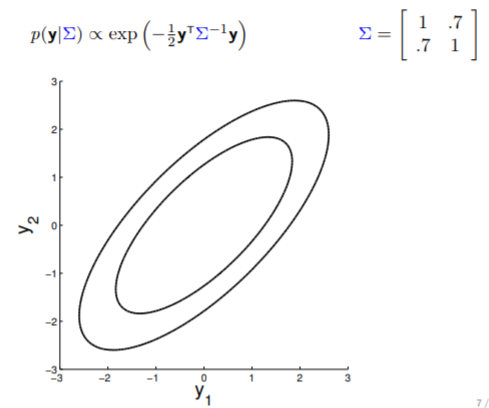
The covariance matrix, denoted as $\Sigma$, tells us (1) the variance of each individual random variable (on diagonal entries) and (2) the covariance between the random variables (off diagonal entries). The covariance matrix in above image indicates that $y_1$ and $y_2$ are positively correlated (with $0.7$ covariance), therefore the somewhat “stretchy” shape of the contour. If we keep reducing the covariance while keeping the variance unchanged, the following transition can be observed:
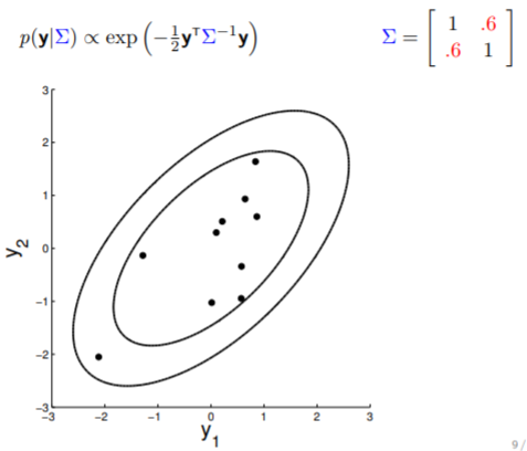
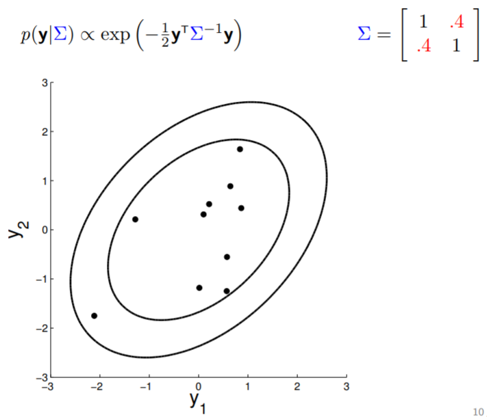
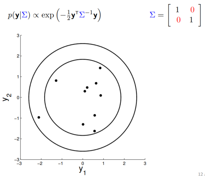
Note that when $y_1$ is independent from $y_2$ (rightmost plot above), the contours are spherical.
Conditioning
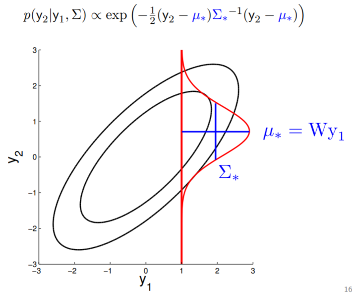
With multivariate Gaussian, another fun thing we can do is conditioning. In 2D, we can demonstrate this graphically:
We fix the value of $y_1$ to compute the density of $y_2$ along the red line – thereby condition on $y_1$. Note that in here since $y_2 \in \mathcal{N}(\mu, \sigma)$ , by conditioning we get a Gaussian back.
We can also visualise how this conditioned gaussian changes as the correlation drop – when correlation is $0$, $y_1$ tells you nothing about $y_2$, so for $y_2$ the mean drop to $0$ and the variance becomes high.
<
High dimensional gaussian: a new interpretation
2D Gaussian
The oval contour graph of Gaussian, while providing information on the mean and covariance of our multivariate Gaussian distribution, does not really give us much intuition on how the random variables correlate with each other during the sampling process.
Therefore, consider this new interpretation that can be plotted as such:
Take the oval contour graph of the 2D Gaussian (left-top in below image) and choose a random point on the graph. Then, plot the value of $y_1$ and $y_2$ of that point on a new graph, at index = $1$ and $2$, respectively.
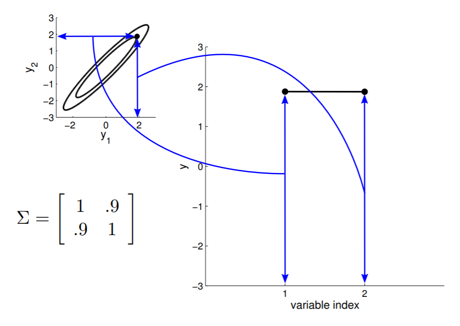
Under this setting, we can now visualise the sampling operation in a new way by taking multiple “random points” and plot $y_1$ and $y_2$ at index $1$ and $2$ multiple times. Because $y_1$ and $y_2$ are correlated ($0.9$ correlation), as we take multiple samples, the bar on the index graph only “wiggles” ever so slightly as the two endpoints move up and down together.
For conditioning, we can simply fix one of the endpoint on the index graph (in below plots, fix $y_1$ to 1) and sample from $y_2$.
Higher dimensional Gaussian
5D Gaussian
Now we can consider a higher dimension Gaussian, starting from 5D — so the covariance matrix is now 5x5.
Take a second to have a good look at the covariance matrix, and notice:
- All variances (diagonal) are equal to 1;
- The further away the indices of two points are, the less correlated they are. For instance, correlation between $y_1$ and $y_2$ is quite high, $y_1$ and $y_3$ lower, $y_1$ and $y_4$ the lowest)
We can again condition on $y_1$ and take samples for all the other points. Notice that $y_2$ is moving less compared to $y_3$ - $y_5$ because it is more correlated to $y_1$.
20D Gaussian
To make things more intuitive, for 20D Gaussian we replace the numerical covariance matrix by a colour map, with warmer colors indicating higher correlation:
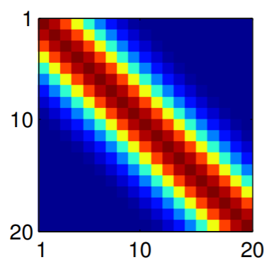
This gives us samples that look like this:
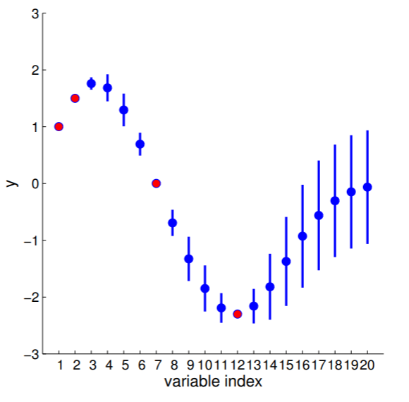
Now look at what happens to the 20D Gaussian conditioned on $y_1$ and $y_2$:
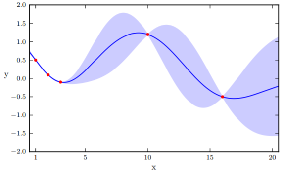
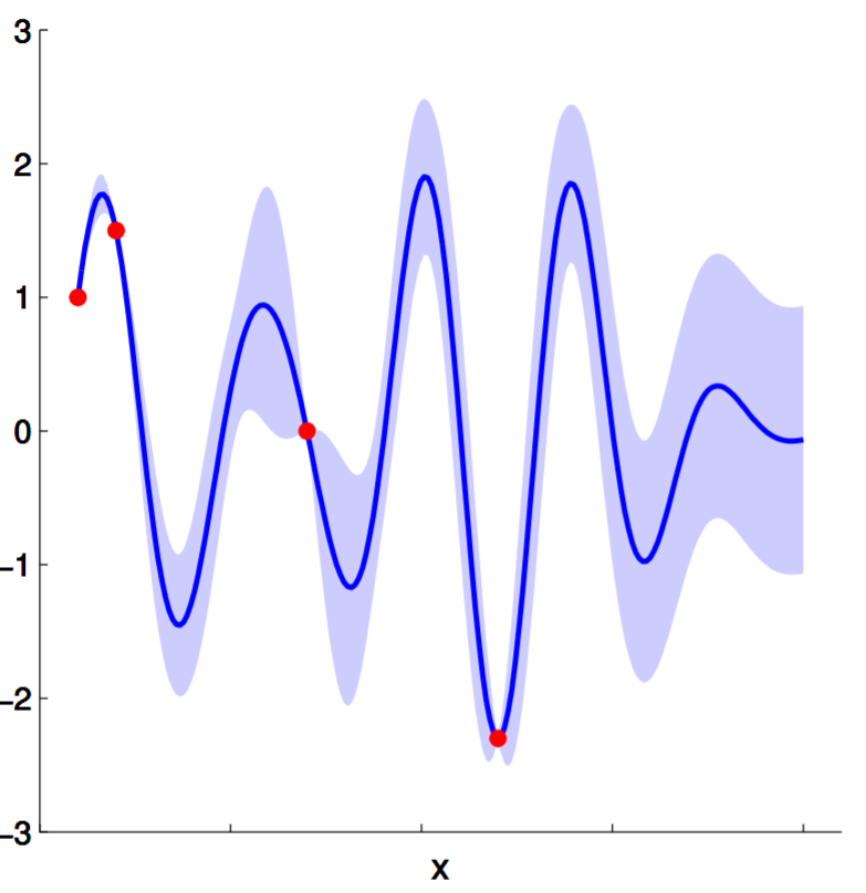
Hopefully you may now be thinking: “Ah, this is looking exactly like the nonlinear regression problem we started with!” And yes, indeed, this is exactly like a nonlinear regression problem where $y_1$ and $y_2$ are given as observations. Using this index plot with 20D Gaussian, we can now generate a family of curves that fits these observations. Even better, if we generate a number of them, we can compute the mean and variance of the fitting using these randomly generated curves. We visualise this in the plot below.
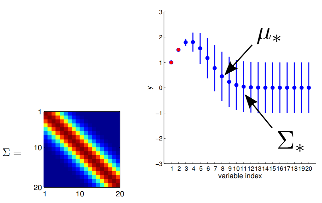
We can see from the above image that because of how covariance matrix is structured (i.e. closer points have higher correlation), the points closer to the observations has very low uncertainty with non-zero mean, whereas the ones further from them have high uncertainty and zero mean. (Note that in reality, we don’t have to actually take many many many samples to estimate the mean and standard deviation, they are completely analytical.)
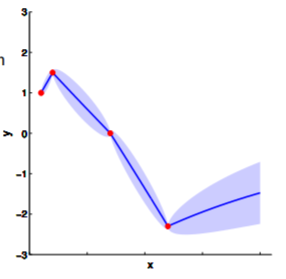
Here we also offer a slightly more exciting example where we condition on 4 points of the 20D Gaussian (and you wonder why everybody hates statisticians):
Getting “real”
The problem with this approach for nonlinear regression seems obvious – it feels like all the points on the x-axis have to be integers because they are indices, while in reality, we want to model observations with real values. One immediately obvious solution for this is, we can keep increasing the dimensionality of the Gaussian and calculate many many points close to the observation, but that is a bit clumsy.
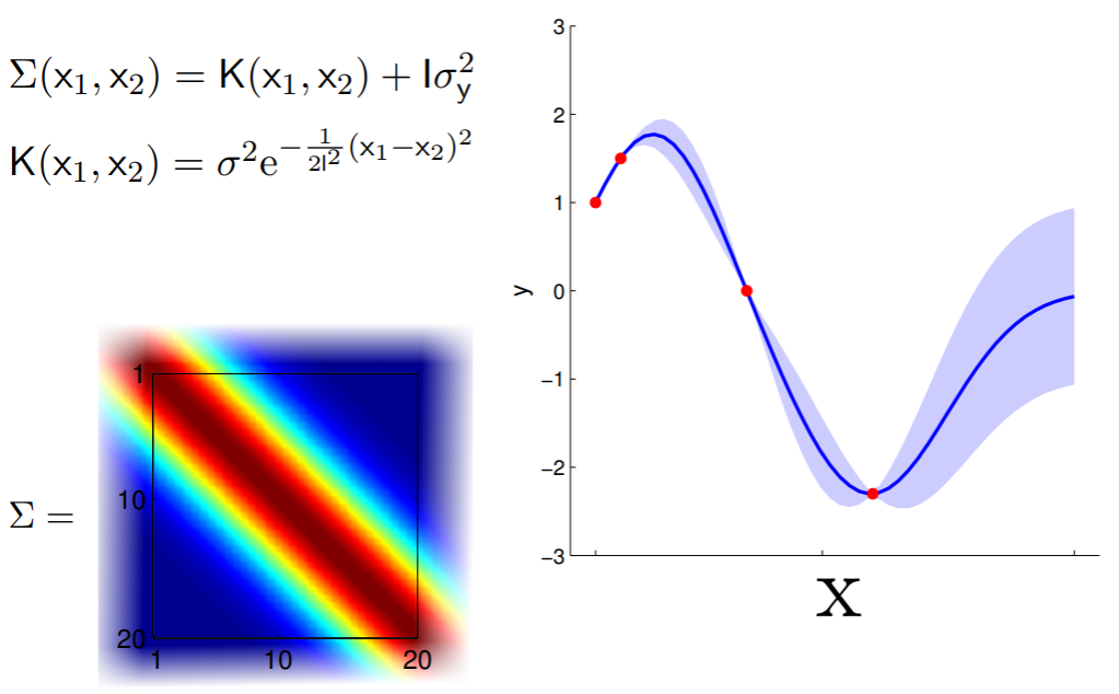
The solution lies in how the covariance matrix is generated. Conventionally, $\Sigma$ is calculated using the following 2-step process:
\(\Sigma (x_1, x_2) = K(x_1, x_2) + I \sigma_y^2\) \(K(x_1, x_2) = \sigma^2 e^{-\frac{1}{2l^2}(x_1 - x_2)^2}\)
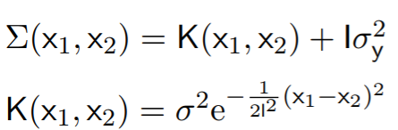
The covariance matrices in all the above examples are computed using the Radial Basis Function (RBF) kernel $K(x_1, x_2)$ – all by taking integer values for $x_1$, $x_2$. This RBF kernel ensures the “smoothness” of the covariance matrix, by generating a large output values for $x_1$, $x_2$ inputs that are closer to each other and smaller values for inputs that are further away . Note that if $x_1=x_2$, $K(x_1, x_2)=\sigma^2$. We then take K and add $I\sigma_y^2$ for the final covariance matrix to factor in noise – more on this later.
This means in principle, we can calculate this covariance matrix for any real-valued $x_1$ and $x_2$ by simply plugging them in. The real-valued $x$s effectively result in an infinite-dimensional Gaussian defined by the covariance matrix.
Now that, is a Gaussian process (mic drop).
Gaussian Process
Textbook definition
From the above derivation, you can view Gaussian process as a generalisation of multivariate Gaussian distribution to infinitely many variables. Here we also provide the textbook definition of GP, in case you had to testify under oath:
A Gaussian process is a collection of random variables, any finite number of which have consistent Gaussian distributions.
Just like a Gaussian distribution is specified by its mean and variance, a Gaussian process is completely defined by (1) a mean function $m(x)$ telling you the mean at any point of the input space and (2) a covariance function $K(x, x’)$ that sets the covariance between points. The mean can be any value and the covariance matrix should be positive definite.
\[f(x) \sim \mathcal{G}\mathcal{P}(m(x), K(x, x'))\]Parametric vs. non-parametric
Note that our Gaussian processes are non-paramatric, as opposed to nonlinear regression models which are parametric. And here’s a secret:
non-parametric model == model with infinite number of parameters

In a parametric model, we define the function explicitly with some parameters:
\[y(x) = f(x) + \epsilon \sigma_y\] \[p(\epsilon) = \mathcal{N}(0,1)\]Where $\sigma_y$ is Gaussian noise describing how noisy the fit is to the actual observation (graphically it’ll represent how often the data lies directly on the fitted curve). We can place a Gaussian process prior over the nonlinear function – meaning, we assume that the parametric function above is drawn from the Gaussian process defined as follow:
\[p(f(x)\mid \theta) = \mathcal{G}\mathcal{P}(0, K(x, x'))\] \[K(x, x') = \sigma^2 \text{exp}(-\frac{1}{2l^2}(x-x')^2)\]This GP will now generate lots of smooth/wiggly functions, and if you think your parametric function falls into this family of functions that GP generates, this is now a sensible way to perform non-linear regression.
We can also add Gaussian noise $\sigma_y$ directly to the model, since the sum of Gaussian variables is also a Gaussian:
\[p(f(x)\mid \theta) = \mathcal{G}\mathcal{P}(0, K(x, x') + I\sigma_y^2)\]In summary, GP regression is exactly the same as regression with parametric models, except you put a prior on the set of functions you’d like to consider for this dataset. The characteristic of this “set of functions” you consider is defined by the kernel of choice ($K(x, x’)$). Note that conventionally the prior has mean 0.
Hyperparameters
There are 2 hyperparameters here:
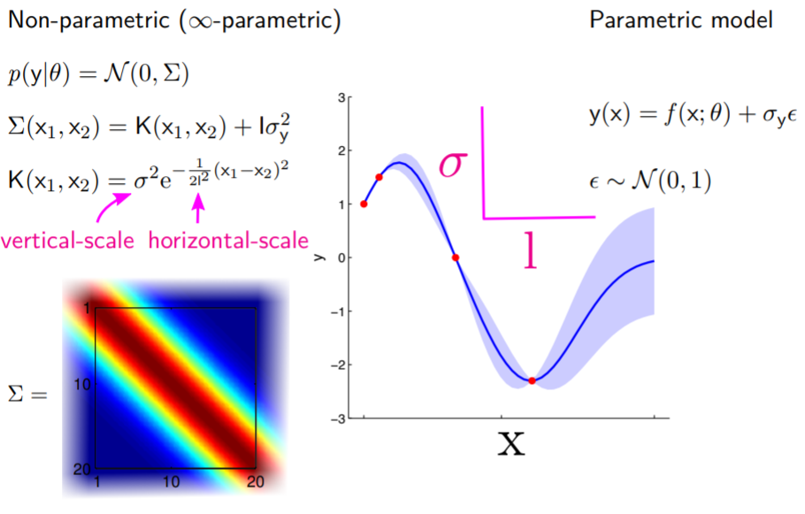
- Vertical scale $\sigma$: describes how much span the function has vertically;
- Horizontal scale $l$: describes how quickly the correlation between two points drops as the distance between them increases – a high $l$ gives you a smooth function, while lower $l$ results in a wiggly function.
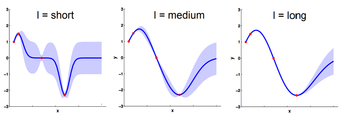
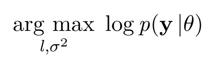
Luckily, because $p(y \mid \theta)$ is Gaussian, we can compute its likelihood in close form. That means we can just maximise the likelihood of $p(y\mid \theta)$ under these hyperparameters using a gradient optimiser:
Details for implementation
Before we start: here we are going to stay quite high level – no code will be shown, but you can easily find many implementations of GP on GitHub (personally I like this repo, it’s a Jupyter Notebook walk through with step-by-step explanation). However, this part is important to understanding how GP actually works, so try not to skip it.
Computation
Hopefully at this point you are wondering: this smooth function with infinite-dimensional covariance matrix thing all sounds well and good, but how do we actually do computation with an infinite by infinite matrix?
Marginalisation baby! Imagine you have a multivariate Gaussian over two vector variables $y_1$ and $y_2$, where:
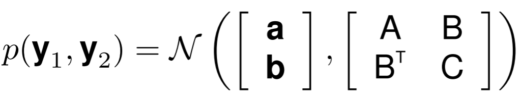
Here, we partition the mean into the mean of $y_1$, $a$ and the mean of $y_2$, $b$; similarly, for covariance matrix, we have $A$ as the covariance of $y_1$, $B$ that of $y_1$ and $y_2$, $B^T$ that of $y_2$ and $y_1$ and $C$ of $y_2$. So now, we can easily compute the probability of $y_1$ using the marginalisation property:
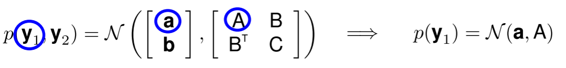
This formation is extremely powerful — it allows us to calculate the likelihood of $y_1$ under the joint distribution of $p(y_1, y_2)$, while completely ignoring $y_2$! We can now generalise from two variables to infinitely many, by altering our definition of $y_1$ and $y_2$ to:
- $y_1$: contains a finite number of variables we are interested in;
- $y_2$: contains all the variables we don’t care about, which is infinitely many; Then similar to the 2-variable case, we can compute the mean and covariance for $y_1$ partition only, without having to worry about the infinite stuff in $y_2$. This nice little property allows us to think about finite dimensional projection of the underlying infinite object on our computer. We can forget about the infinite stuff happening under the hood.
Predictions
Taking the above $y_1$, $y_2$ example, but this time imagine all the observations are in partition $y_2$ and all the points we want to make predictions about are in $y_1$ (again, the infinite points are still in the background, let’s imagine we’ve shoved them into some $y_3$ that is omitted here).
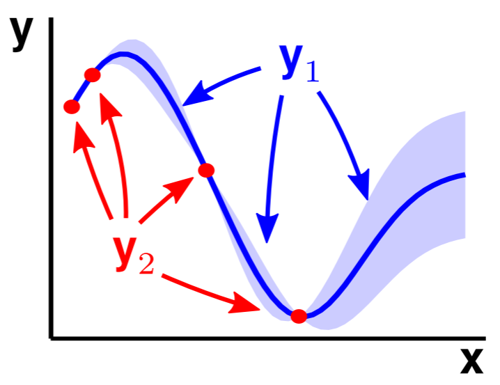
To make predictions about $y_1$ given observations of $y_2$, we can then use bayes rules to calculate $p(y_1\mid y_2)$:
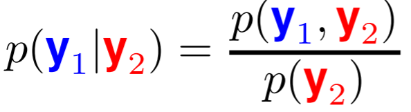
Because $p(y_1)$, $p(y_2)$ and $p(y_1,y_2)$ are all Gaussians, $p(y_1\mid y_2)$ is also Gaussian. We can therefore compute $p(y_1\mid y_2)$ analytically:
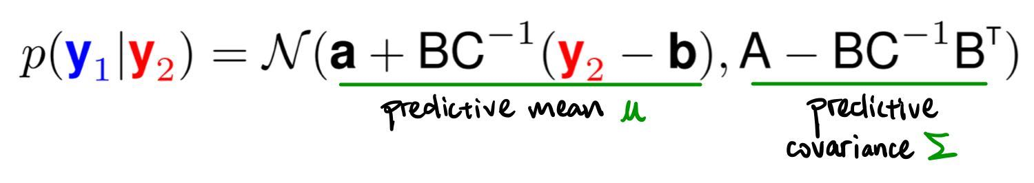
Note: here we catch a glimpse of the bottleneck of GP: we can see that this analytical solution involves computing the inverse of the covariance matrix of our observation $C^{-1}$, which, given $n$ observations, is an $O(n^3)$ operation. This is why we use Cholesky decomposition – more on this later.
To gain some more intuition on the method, we can write out the predictive mean and predictive covariance as such:
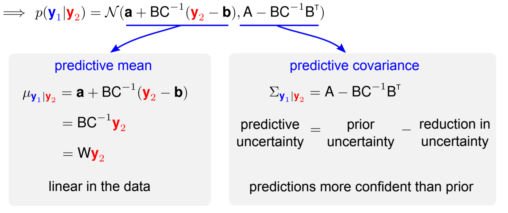
So the mean of $p(y_1 \mid y_2)$ is linearly related to $y_2$, and the predictive covariance is the prior uncertainty subtracted by the reduction in uncertainty after seeing the observations. Therefore, the more data we see, the more certain we are.
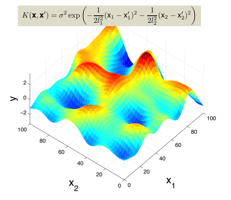
Higher dimensional data
You can also do this for higher-dimensional data (though of course at greater computational costs). Here we extend the covariance function to incorporate RBF kernels in 2D data:
Covariance matrix selection
As one last detail, let’s talk about the different covariance matrices used for GP. I don’t have any authoritative advice on selecting kernels for GP in general, and I believe in practice, most people try a few popular kernels and pick the one that fits their data/problem the best. So here we will only introduce the form of some of the most frequently seen kernels, get a feel for them with some plots and not go into too much detail. (I highly recommend implementing some of them and play around with it though! It’s good coding practice and best way to gain intuitions about these kernels.)
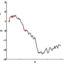
Laplacian Function
This function is continuous but non-differentiable. It looks like this:
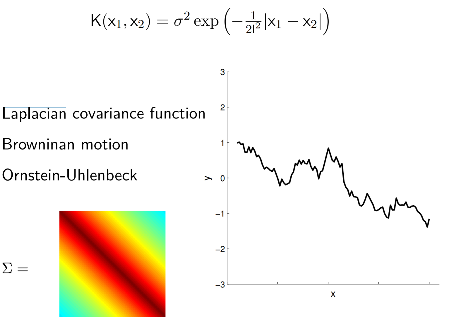
If you average over all samples, you get straight lines joining your datapoints, which are called Browninan bridges.
Rational quadratic
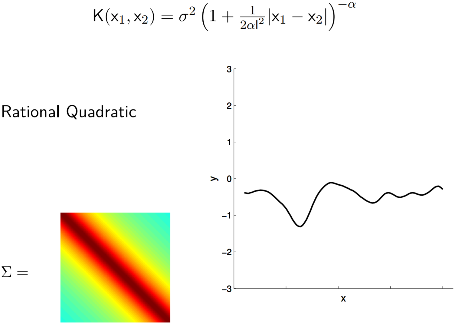
Average over all samples looks like this:

Periodic functions
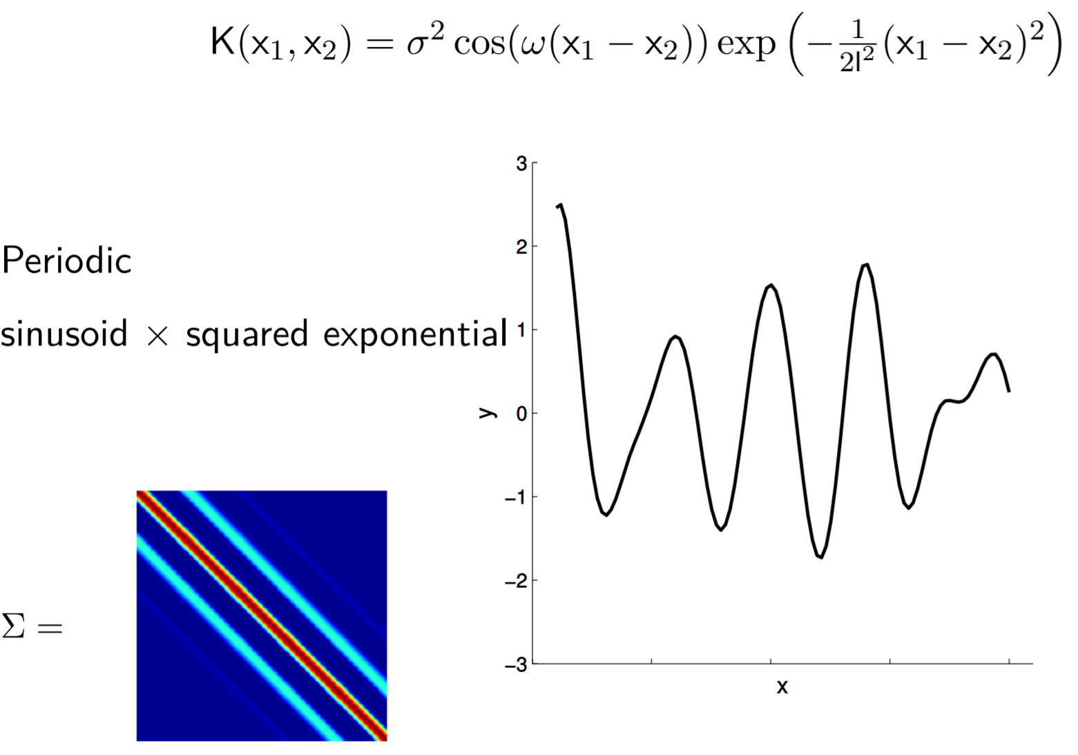
Average over all samples looks like this:
Summary
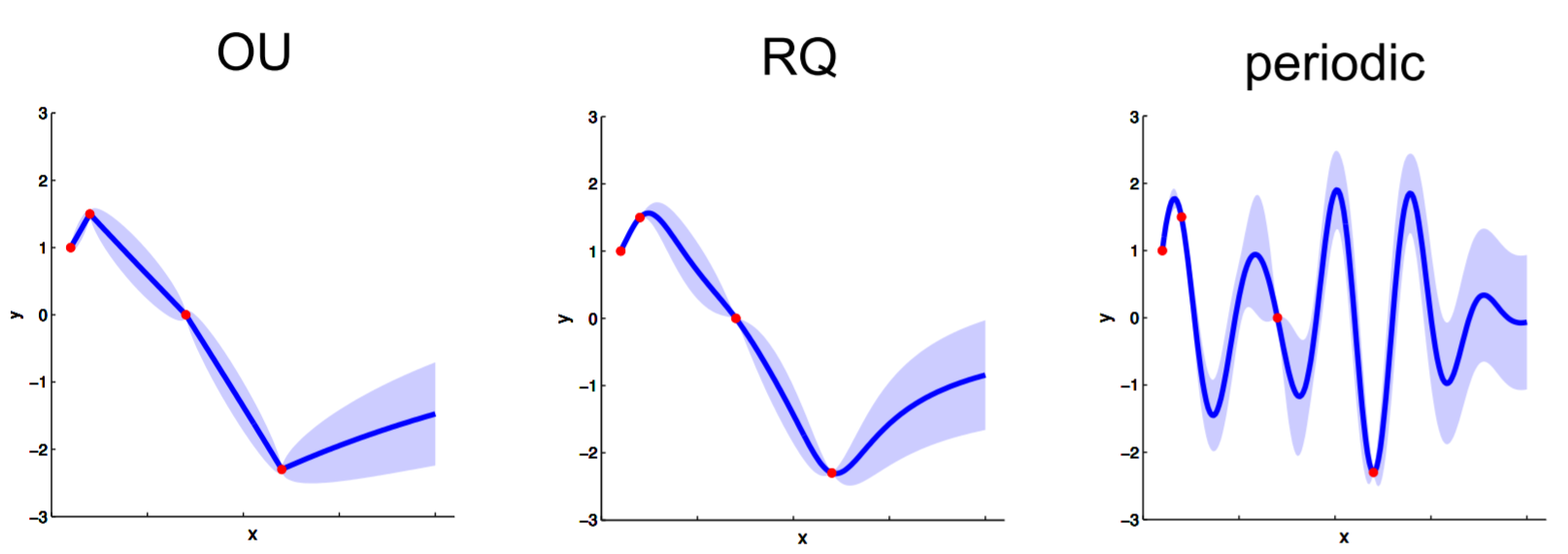
There are books that you can look up for appropriate kernels for covariance functions for your particular problem, and rules you can follow to produce more complicated covariance functions (such as, the product of two covariance functions is a valid covariance function). They can give you very different results:
It is tricky to find the appropriate covariance function, but there are also methods in place for model selection. One of those methods is Bayesian model comparison, defined as follows:
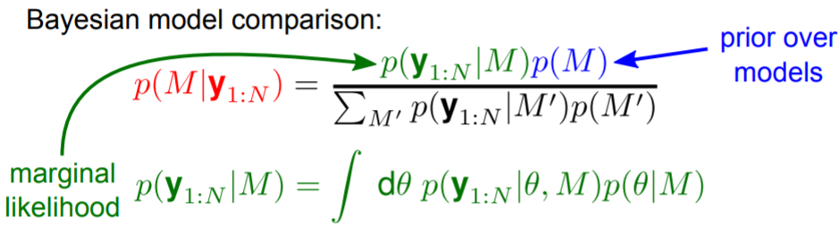
However, it does involve a very difficult integral (or sum in discrete case, as showed above) over the hyperparameters of your GP, which makes it impractical, and is also very sensitive to the prior you put over your hyperparameters. In practice, it is more common to use deep Gaussian Processes for automatic kernel design, which optimises the choice of covariance function that is appropriate for your data through training.
The end
Hopefully this has been a helpful guide to Gaussian process for you. I want to keep things relatively short and simple here, so I did not delve into the complications of using GPs in practice – in reality GPs suffers from not being able to scale to large datasets, and the choice of kernels can be very tricky. There are some state-of-the-art approaches that tackle with these issues (see deep GP and sparse GP), but since I am by no means an expert in this area I will leave you to exploring them.
Thank you for reading! Remember to take your canvas bag to the supermarket, baby whales are dying.

Acknowledgements
I would like to thank Andrey Kurenkov and Hugh Zhang from The Gradient for helping me with the edits of this article.
Leave a Comment